Deep Dive Part 1: Wrestling Climate Data Into Submission

In my previous post, I shared the high-level story of predicting wine grape suitability under climate change. Now, let's get technical.

If you've ever worked on a real-world ML project, you know the dirty secret: data collection and cleaning consume 70-80% of your time. This project was no exception. In fact, data wrangling was so involved that I broke my Jupyter notebooks into five separate data collection notebooks before I could even start exploratory analysis.

Here's how I turned scattered climate observations into a clean, analysis-ready dataset — and the lessons I learned along the way.

The Data Requirements: What Does "Suitable Climate" Actually Mean?

Before diving into data sources, I needed to define what climate features matter for wine grape suitability. This required research into viticulture science.

Grapes are sensitive to:

• Temperature: Both total accumulated heat and extreme events
• Precipitation: Seasonal patterns matter more than annual totals
• Temperature variability: Day-night swings affect phenolic development
• Frost risk: Late spring frosts can devastate a harvest
• Growing season length: Days between frost dates

Armed with this domain knowledge, I identified the raw climate variables I needed:

• Daily minimum and maximum temperature
• Daily precipitation
• Derived indices: Growing Degree Days, Winkler Index, Cool Night Index

And I needed them for:

• Geographic coverage: Six wine regions across California and France
• Temporal coverage: 27 years (2000-2026) to capture climate variability
• Spatial resolution: Fine enough to distinguish between neighboring regions

Now came the fun part: finding this data.

Data Source 1: PRISM Climate Group (California)

For California regions (Anderson Valley, Napa, Russian River, Sonoma, Paso Robles), I used the PRISM Climate Group dataset from Oregon State University.

Why PRISM?

• High spatial resolution: 800-meter grids (roughly 0.5 miles)
• Accounts for terrain effects on climate (crucial for mountainous wine regions)
• Available daily data back to 1981
• Free for research use

The catch? PRISM data comes in netCDF4 format — multidimensional arrays that store spatial climate grids over time. If you've never worked with netCDF, imagine a 3D cube: latitude × longitude × time.

Code: Extracting PRISM Data

import xarray as xr
import numpy as np
import pandas as pd
from pathlib import Path

def extract_prism_region(netcdf_path, region_bounds, variable='tmax'):
    """
    Extract time series for a wine region from PRISM netCDF files.

    Parameters:
    -----------
    netcdf_path : Path to PRISM netCDF file
    region_bounds : dict with 'lat_min', 'lat_max', 'lon_min', 'lon_max'
    variable : 'tmax', 'tmin', or 'ppt'

    Returns:
    --------
    pd.DataFrame with daily values averaged over the region
    """
    # Open the netCDF dataset
    ds = xr.open_dataset(netcdf_path)

    # Select the region (PRISM uses negative longitude for western hemisphere)
    region = ds.sel(
        lat=slice(region_bounds['lat_min'], region_bounds['lat_max']),
        lon=slice(region_bounds['lon_min'], region_bounds['lon_max'])
    )

    # Spatial average over the region
    region_mean = region[variable].mean(dim=['lat', 'lon'])

    # Convert to pandas DataFrame
    df = region_mean.to_dataframe().reset_index()
    df['region'] = region_bounds['name']

    return df[['time', 'region', variable]]

# Example: Napa Valley bounds
napa_bounds = {
    'name': 'Napa Valley',
    'lat_min': 38.2,
    'lat_max': 38.8,
    'lon_min': -122.6,
    'lon_max': -122.2
}

# Extract temperature data
napa_tmax = extract_prism_region(
    'data/raw/prism_tmax_2000_2026.nc',
    napa_bounds,
    variable='tmax'
)

Challenge 1: Geographic Boundary Definition

How do you define "Napa Valley" in lat/lon coordinates? Wine regions don't have precise boundaries — they're cultural and agricultural designations, not geographic polygons.

My approach:

1. Research AVA (American Viticultural Area) boundaries from TTB (Alcohol and Tobacco Tax and Trade Bureau)
2. Cross-reference with Google Maps to identify vineyard concentrations
3. Create conservative bounding boxes that capture core production areas
4. Validate by comparing climate statistics to published viticulture literature

For example, Napa Valley's primary vineyard areas span roughly:

• Latitude: 38.2°N to 38.8°N
• Longitude: -122.6°W to -122.2°W

This captures the valley floor and lower hillsides where most production occurs.

Challenge 2: Temporal Alignment

PRISM data is daily, but wine regions need annual summaries. A "year" in viticulture isn't January-December — it's growing season (April-October in Northern Hemisphere) or vintage year.

I created two temporal aggregations:

• Calendar year: Jan 1 - Dec 31 (for dormant season precipitation)
• Growing season: April 1 - October 31 (for GDD, extreme heat)

def aggregate_to_annual(daily_df, variable, region):
    """
    Aggregate daily climate data to annual summaries.
    """
    # Extract year from datetime
    daily_df['year'] = pd.to_datetime(daily_df['time']).dt.year
    daily_df['month'] = pd.to_datetime(daily_df['time']).dt.month

    # Define growing season (April-October)
    daily_df['growing_season'] = daily_df['month'].isin(range(4, 11))

    # Annual aggregations
    annual = daily_df.groupby('year').agg({
        variable: ['mean', 'max', 'min', 'std'],
    })

    # Growing season aggregations
    growing = daily_df[daily_df['growing_season']].groupby('year').agg({
        variable: ['mean', 'max'],
    })

    return annual, growing

Data Source 2: European Climate Assessment & Dataset (ECA&D)

For the Rhône Valley reference region, I used ECA&D, which provides long-term European climate observations.

Key differences from PRISM:

• Station-based observations (not gridded)
• Different file format (text with custom headers)
• Missing data coded as -9999
• Quality flags need filtering

Code: Parsing ECA&D Station Data

def parse_ecad_station(file_path):
    """
    Parse ECA&D station file with custom header format.
    """
    # ECA&D files have 20-line headers
    df = pd.read_csv(
        file_path,
        skiprows=20,
        sep=',',
        names=['STAID', 'SOUID', 'DATE', 'VALUE', 'Q_FLAG']
    )

    # Remove missing data (-9999) and quality-flagged observations
    df = df[(df['VALUE'] != -9999) & (df['Q_FLAG'] == 0)]

    # ECA&D stores temperature in 0.1°C units
    df['VALUE'] = df['VALUE'] / 10.0

    # Parse date (format: YYYYMMDD)
    df['DATE'] = pd.to_datetime(df['DATE'], format='%Y%m%d')

    return df[['DATE', 'VALUE']]

# For Rhône Valley, I averaged 3 stations:
# - Orange (primary wine region)
# - Avignon
# - Montélimar

Challenge 3: Spatial Aggregation from Stations

Unlike PRISM's grids, ECA&D provides point observations at weather stations. To get a regional average, I needed to:

1. Identify stations within the Rhône Valley wine region
2. Quality-filter observations
3. Average across stations (weighted by data completeness)

def aggregate_stations(station_files, region_name):
    """
    Combine multiple weather stations into regional average.
    """
    all_data = []

    for station_file in station_files:
        df = parse_ecad_station(station_file)
        df['station'] = station_file.stem  # filename as station ID
        all_data.append(df)

    # Combine all stations
    combined = pd.concat(all_data)

    # Daily average across stations
    regional = combined.groupby('DATE')['VALUE'].mean().reset_index()
    regional['region'] = region_name

    return regional

Data Source 3: Climate Projections (CMIP6)

For 2050 projections, I used downscaled CMIP6 climate models — specifically the SSP2-4.5 scenario (moderate emissions pathway).

Why SSP2-4.5?

• Represents a "middle of the road" scenario
• Assumes some climate policy but not aggressive mitigation
• Projects global warming of ~2.5°C by 2050 (relative to pre-industrial)

Regional projections used:

• Anderson Valley: +2.0°C
• Napa Valley: +2.5°C
• Russian River: +2.2°C (coastal buffering)
• Sonoma: +2.3°C
• Paso Robles: +2.8°C (inland warming)

These aren't uniform — coastal regions warm more slowly due to ocean influence, inland valleys warm faster.

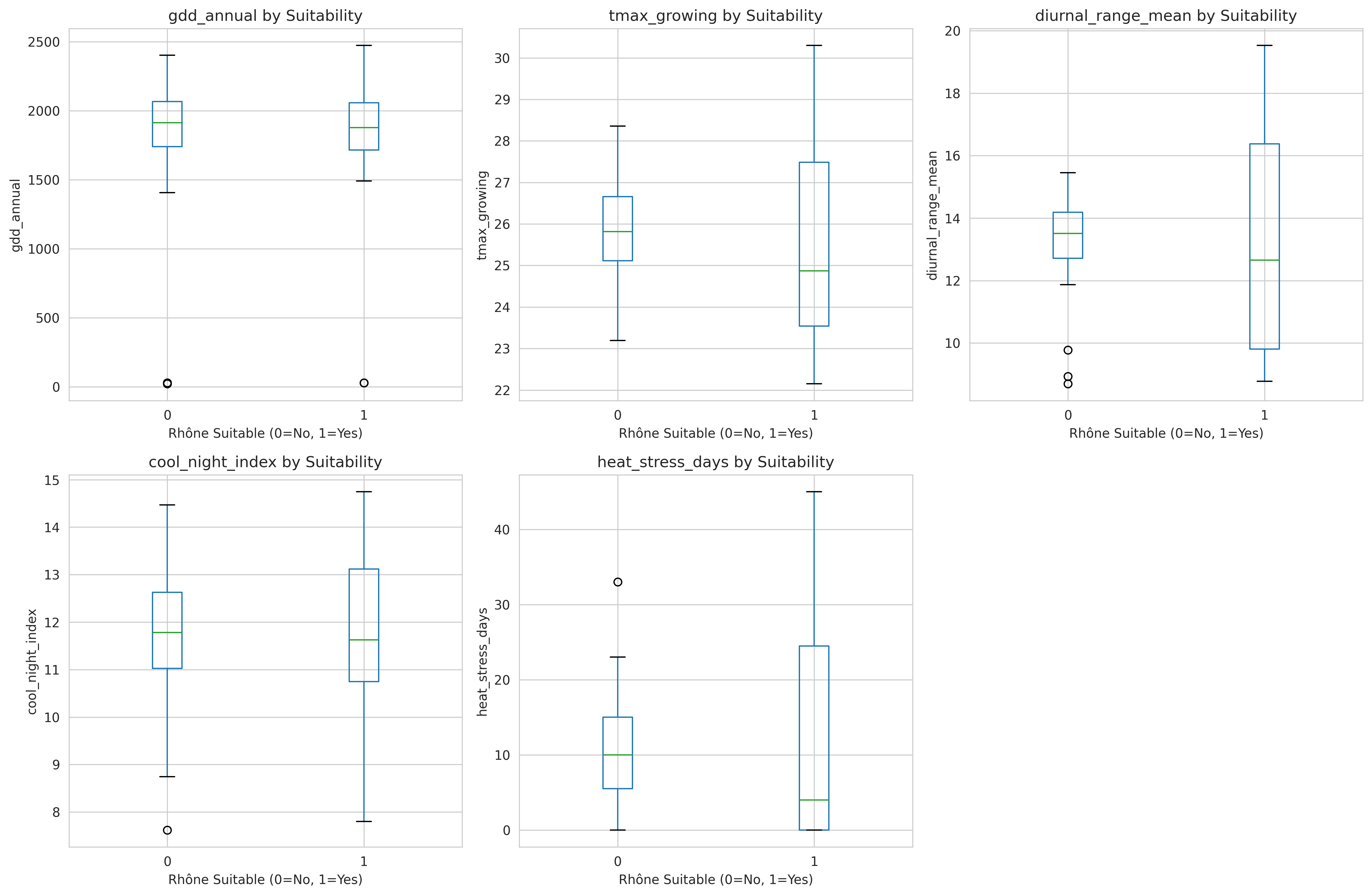
Feature Engineering: From Raw Data to Viticulture Indices

With raw temperature and precipitation data in hand, I engineered 26 climate features. Here are the most important:

Growing Degree Days (GDD)

The classic viticulture metric: accumulated heat above a base temperature.

def calculate_gdd(daily_temps, base_temp=10):
    """
    Calculate Growing Degree Days.
    Formula: GDD = max(0, (Tmax + Tmin)/2 - base_temp)

    Parameters:
    -----------
    daily_temps : DataFrame with 'tmax' and 'tmin' columns
    base_temp : Base temperature in Celsius (10°C for grapevines)
    """
    daily_temps['tavg'] = (daily_temps['tmax'] + daily_temps['tmin']) / 2
    daily_temps['gdd'] = (daily_temps['tavg'] - base_temp).clip(lower=0)

    # Annual sum
    annual_gdd = daily_temps.groupby('year')['gdd'].sum()

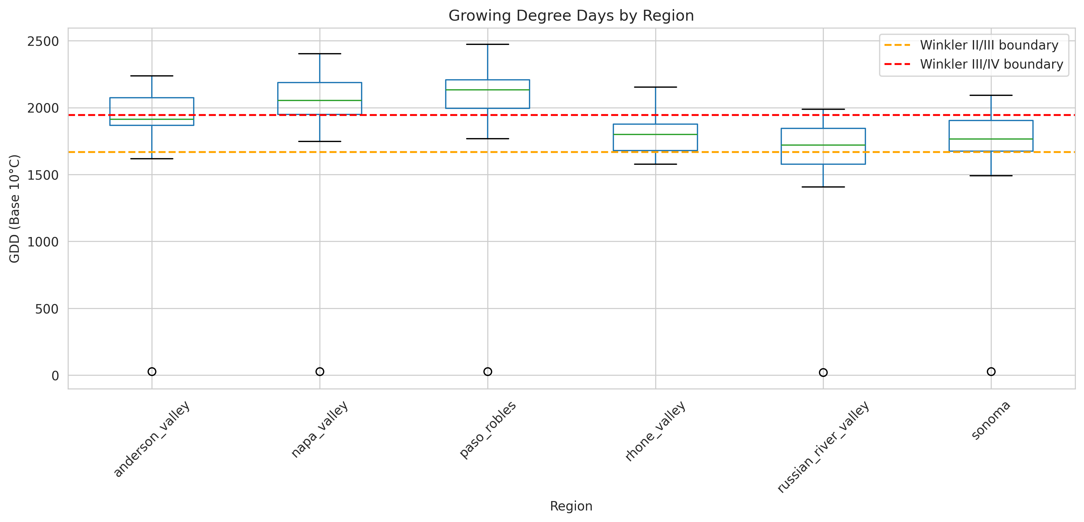
    return annual_gdd

Typical ranges:

• Anderson Valley: 1,800-2,000 GDD (cool climate)
• Napa Valley: 2,000-2,400 GDD (moderate)
• Paso Robles: 2,400-2,800 GDD (warm climate)
• Rhône Valley: 1,800-2,200 GDD (reference)

Extreme Heat Metrics

GDD misses important extremes. I added:

def calculate_extreme_heat(daily_temps):
    """
    Calculate extreme heat metrics.
    """
    metrics = {}

    # 95th percentile maximum temperature
    metrics['tmax_p95'] = daily_temps['tmax'].quantile(0.95)

    # Heat stress days (consecutive days above 35°C)
    heat_stress = (daily_temps['tmax'] > 35).astype(int)
    metrics['heat_stress_days'] = heat_stress.sum()

    # Maximum consecutive hot days
    metrics['max_heat_wave'] = (
        heat_stress.groupby((heat_stress != heat_stress.shift()).cumsum())
        .sum()
        .max()
    )

    return pd.Series(metrics)

Diurnal Temperature Range

The day-night temperature swing is crucial for phenolic compound development (color and tannins in red wine).

def calculate_diurnal_range(daily_temps):
    """
    Calculate average diurnal temperature range.
    """
    daily_temps['diurnal_range'] = daily_temps['tmax'] - daily_temps['tmin']

    return daily_temps.groupby('year')['diurnal_range'].mean()

Rhône varieties prefer high diurnal ranges (15-20°C) — hot days for sugar accumulation, cool nights for acid retention.

Precipitation Patterns

Wine grapes need Mediterranean-style precipitation: wet winters, dry summers.

def calculate_precipitation_metrics(daily_precip):
    """
    Calculate viticulture-relevant precipitation metrics.
    """
    # Add month column
    daily_precip['month'] = pd.to_datetime(daily_precip['time']).dt.month

    metrics = {}

    # Dormant season (November-March)
    dormant = daily_precip[daily_precip['month'].isin([11, 12, 1, 2, 3])]
    metrics['ppt_dormant'] = dormant.groupby('year')['ppt'].sum()

    # Growing season (April-October)
    growing = daily_precip[daily_precip['month'].isin(range(4, 11))]
    metrics['ppt_growing'] = growing.groupby('year')['ppt'].sum()

    # Mediterranean ratio (dormant / growing)
    metrics['med_ratio'] = metrics['ppt_dormant'] / metrics['ppt_growing']

    # Precipitation variability (CV)
    annual = daily_precip.groupby('year')['ppt'].sum()
    metrics['ppt_cv'] = annual.std() / annual.mean()

    return pd.DataFrame(metrics)

Target pattern for Rhône varieties:

• Dormant season: 400-600mm (winter rain recharges soil)
• Growing season: 100-200mm (dry summers reduce disease)
• Mediterranean ratio: 2.5-4.0 (3x more rain in winter than summer)

Data Quality Control

Real-world data is messy. Here's how I handled quality issues:

1. Missing Data

def check_data_completeness(df, threshold=0.95):
    """
    Flag years with insufficient data coverage.
    """
    # Count valid observations per year
    coverage = df.groupby('year')['value'].count() / 365

    # Flag incomplete years
    incomplete_years = coverage[coverage < threshold].index

    if len(incomplete_years) > 0:
        print(f"Warning: {len(incomplete_years)} years below {threshold*100}% coverage")
        print(incomplete_years.tolist())

    return df[~df['year'].isin(incomplete_years)]

I removed years with <95% data coverage. This eliminated:

• 2001 for Russian River (station malfunction)
• 2015 for Rhône Valley (data gap during station upgrade)

2. Outlier Detection

def flag_outliers(df, variable, n_std=3):
    """
    Flag statistical outliers using z-score method.
    """
    z_scores = np.abs((df[variable] - df[variable].mean()) / df[variable].std())
    outliers = df[z_scores > n_std]

    if len(outliers) > 0:
        print(f"Found {len(outliers)} outliers for {variable}")
        print(outliers[['date', variable]])

    return z_scores > n_std

Flagged but didn't automatically remove outliers — extreme weather events (heat waves, cold snaps) are real and relevant to climate analysis.

3. Cross-Validation with Published Data

I validated my processed data against published climate summaries:

• UC Davis viticulture reports
• NOAA Climate Division summaries
• French National Weather Service (Météo-France)

Example validation:

My calculation: Napa Valley 2000-2010 average GDD = 2,147
UC Davis report: Napa Valley 2000-2010 average GDD = 2,156
Difference: -0.4% ✓

The Final Dataset

After all this wrangling, I had:

Structure:

• 130 observations (27 years × 6 regions, minus incomplete years)
• 26 climate features
• 1 binary label (suitable/unsuitable for Rhône varieties)

File organization:

data/
├── raw/                          # Original downloads
│   ├── prism/
│   │   ├── tmax_2000_2026.nc
│   │   ├── tmin_2000_2026.nc
│   │   └── ppt_2000_2026.nc
│   └── ecad/
│       ├── orange_station.txt
│       └── avignon_station.txt
├── interim/                      # Intermediate processing
│   ├── daily_regional_temps.csv
│   └── daily_regional_precip.csv
└── processed/                    # Analysis-ready
    ├── climate_features_annual.csv
    └── climate_features_metadata.json

Key Lessons from Data Collection

1. Invest time in understanding data formats

I spent a full week just learning netCDF4 manipulation. That upfront investment paid off when I needed to extract data for multiple regions and variables.

2. Validate early and often

Comparing my calculations to published summaries caught several unit conversion errors (°F vs °C, mm vs inches) before they poisoned downstream analysis.

3. Document everything

I created a data_sources.md file documenting every data source URL, download dates, processing steps, and known limitations. Six months later, I was grateful for this documentation.

4. Domain knowledge prevents costly mistakes

Understanding that wine regions care about growing season vs calendar year saved me from engineering features that would be meaningless to viticulturists.

5. Automate what you'll repeat

I wrapped repetitive tasks (region extraction, feature calculation) into reusable functions. When I later added Anderson Valley as a sixth region, I just updated a config file instead of rewriting code.

Code Repository: All data processing code is available in notebooks/01a-01e_data_collection.ipynb and modularized in src/data/ on GitHub.