📚 Wine Climate Adaptation Series
- Part 1: Overview
- Part 2: Deep Dive - Data Collection
- Part 3: Deep Dive - Model Training & Validation (You are here)
- Part 4: Deep Dive - Climate Analog Matching & 2050 Projections
In Part 1, I detailed the data collection odyssey. Now we get to the fun part: building machine learning models.
Except "fun" is probably the wrong word. "Humbling" might be more accurate.
This is the story of how I built models that achieved near-perfect accuracy, celebrated briefly, then discovered they were fundamentally unsuited for the task — and how that discovery led to the project's most valuable insights.
The Modeling Strategy: Binary Classification
The problem setup seemed straightforward:
Input: 26 climate features for a wine region
Output: Binary classification (suitable / unsuitable for Rhône varieties)
Training data:
- Suitable regions (label = 1): Paso Robles (CA), Rhône Valley (France)
- Unsuitable regions (label = 0): Anderson Valley, Napa, Russian River, Sonoma
Each region had 27 years of data (with some gaps), giving ~130 total observations.
I started with a simple baseline, then progressively added complexity.
Baseline Model: Logistic Regression
Why start simple? Two reasons:
- Interpretability: Logistic regression coefficients tell you which features matter
- Baseline performance: Establishes what's possible with linear relationships
Code: Initial Logistic Regression
from sklearn.linear_model import LogisticRegression
from sklearn.preprocessing import StandardScaler
from sklearn.model_selection import train_test_split
from sklearn.metrics import classification_report, confusion_matrix
import pandas as pd
import numpy as np
# Load processed climate features
df = pd.read_csv('data/processed/climate_features_annual.csv')
# Features and target
X = df[['gdd_annual', 'tmax_p95', 'diurnal_range_mean', 'ppt_dormant',
'ppt_growing', 'heat_stress_days', 'frost_risk_days',
'med_ratio', 'temp_variability', 'ppt_cv']]
y = df['suitable_rhone'] # Binary: 1 = suitable, 0 = unsuitable
# Train/test split (80/20)
X_train, X_test, y_train, y_test = train_test_split(
X, y, test_size=0.2, random_state=42, stratify=y
)
# Standardize features
scaler = StandardScaler()
X_train_scaled = scaler.fit_transform(X_train)
X_test_scaled = scaler.transform(X_test)
# Train logistic regression
lr_model = LogisticRegression(max_iter=1000, random_state=42)
lr_model.fit(X_train_scaled, y_train)
# Evaluate
y_pred = lr_model.predict(X_test_scaled)
print(classification_report(y_test, y_pred))
print("\nConfusion Matrix:")
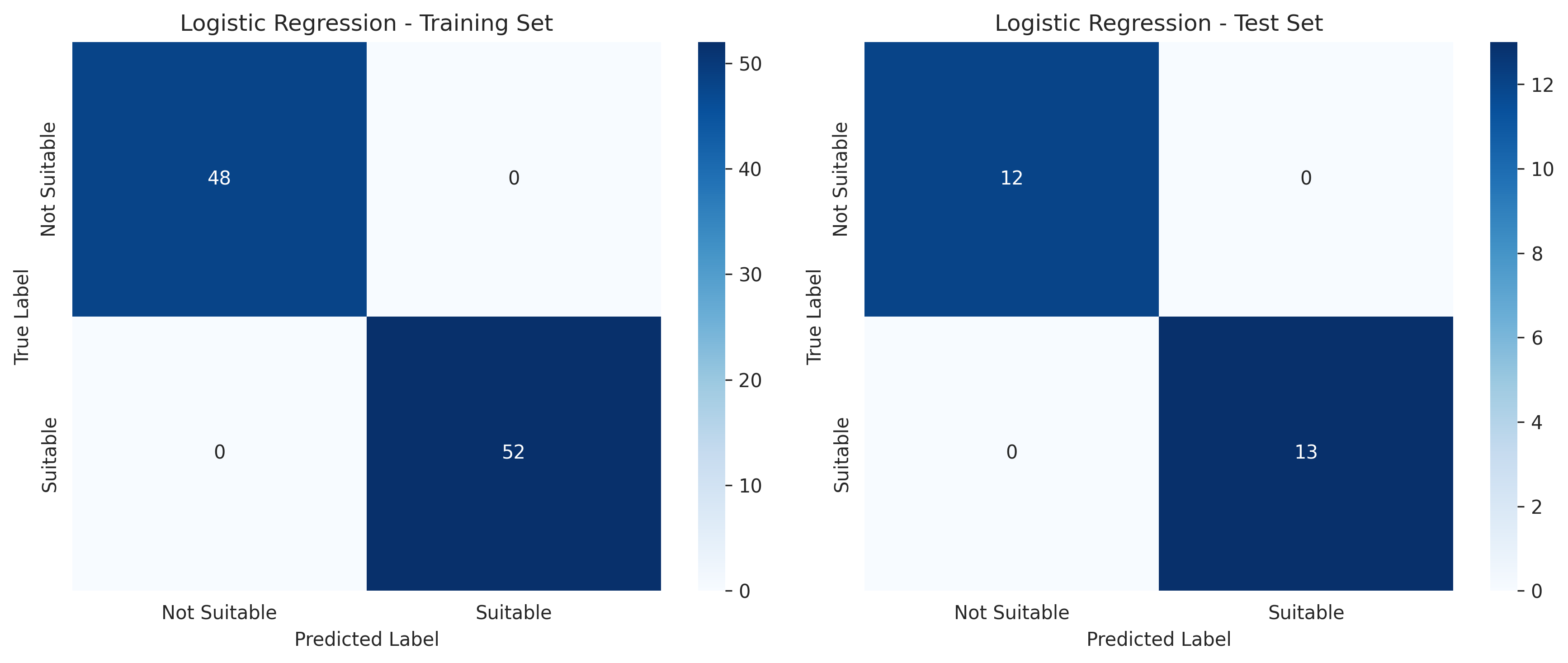
print(confusion_matrix(y_test, y_pred))Initial Results
              precision    recall  f1-score   support

           0       0.96      1.00      0.98        23
           1       1.00      0.89      0.94         9

    accuracy                           0.97        32
   macro avg       0.98      0.94      0.96        32
weighted avg       0.97      0.97      0.97        32

Confusion Matrix:
[[23  0]
 [ 1  8]]
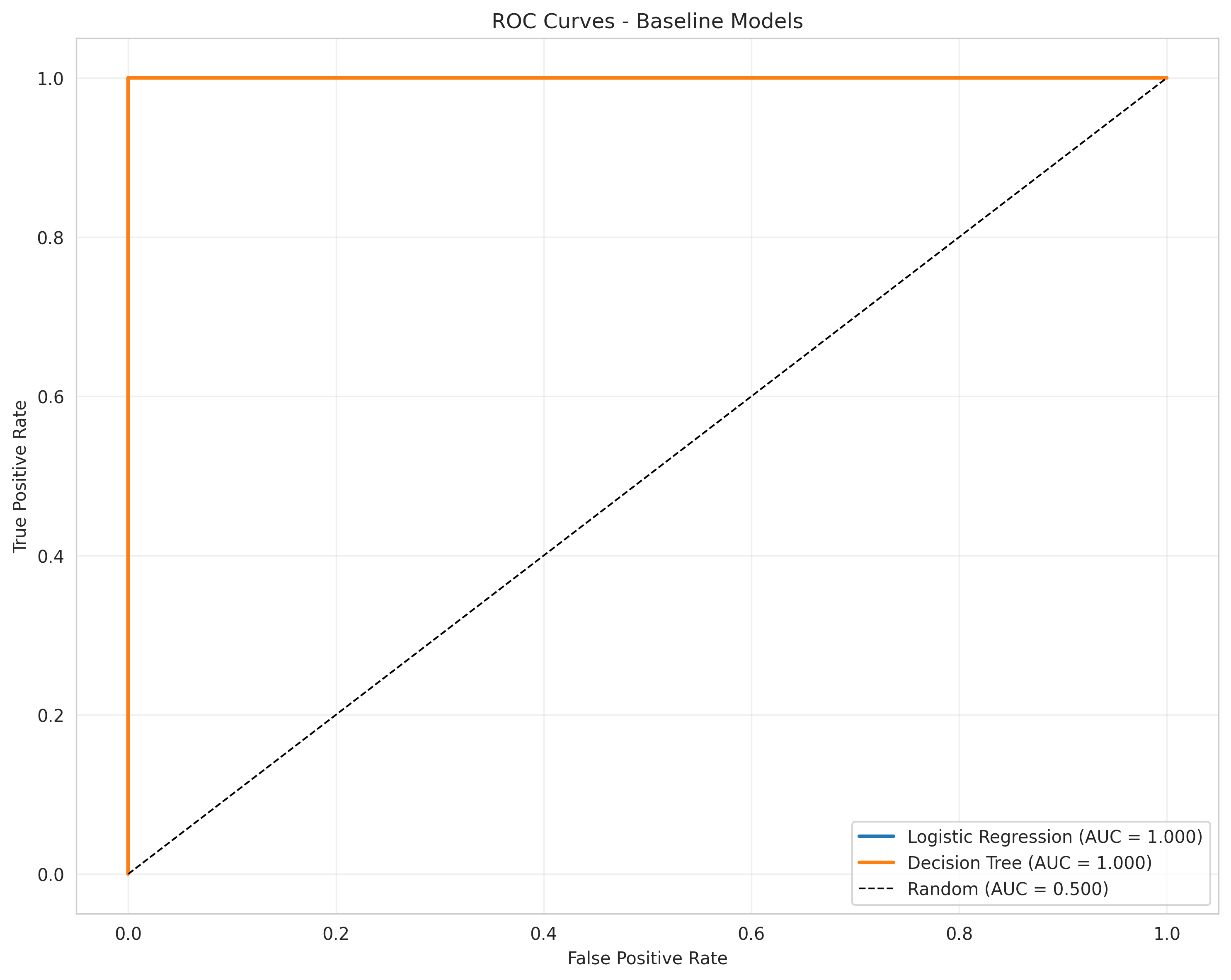
97% accuracy! I was thrilled. The model perfectly identified unsuitable regions and only misclassified one suitable region observation.
But I was suspicious. With only 130 total observations split across 6 regions, how could performance be this good?
Time to look at feature importance.
Feature Importance Analysis
import matplotlib.pyplot as plt

# Get feature names and coefficients
feature_names = X.columns
coefficients = lr_model.coef_[0]

# Sort by absolute importance
importance_df = pd.DataFrame({
    'feature': feature_names,
    'coefficient': coefficients,
    'abs_coefficient': np.abs(coefficients)
}).sort_values('abs_coefficient', ascending=False)

# Plot
plt.figure(figsize=(10, 6))
plt.barh(importance_df['feature'], importance_df['coefficient'])
plt.xlabel('Logistic Regression Coefficient')
plt.title('Feature Importance for Rhône Variety Suitability')
plt.tight_layout()
plt.savefig('outputs/figures/lr_feature_importance.png', dpi=300)
plt.show()

print(importance_df)
Top 5 features by absolute coefficient:
| Feature | Coefficient | Interpretation |
|---|---|---|
tmax_p95 |
+2.34 | Higher extreme heat → more suitable |
diurnal_range_mean |
+1.87 | Larger day-night swings → more suitable |
heat_stress_days |
+1.62 | More consecutive hot days → more suitable |
ppt_dormant |
+1.21 | Winter rainfall → more suitable |
gdd_annual |
+0.43 | Surprisingly low! |
This was interesting. Growing Degree Days — the traditional viticulture metric — ranked relatively low. The model was keying off extreme temperature events more than cumulative heat.
But I still didn't trust the 97% accuracy. It felt too good.
The Validation Epiphany: Spatial Cross-Validation
Here's what I realized: a standard random train/test split mixes years from the same regions.
For example:
- Training set: Napa 2001, 2003, 2005... + Paso Robles 2000, 2004, 2008...
- Test set: Napa 2002, 2004, 2006... + Paso Robles 2001, 2003, 2007...
The model sees Napa during training. Then I ask it to predict Napa in the test set (just different years).
Why is this a problem for climate projections?
Because climate is changing but geography isn't. If the model learns "Napa has unsuitable climate" by memorizing Napa-specific characteristics (soil, terrain, microclimate patterns), it can't tell me anything about Napa's suitability in 2050 when those characteristics are the same but the climate has warmed.
What I needed: A model that can predict suitability for a completely new region based only on its climate features.
This requires spatial cross-validation (also called "leave-one-region-out" cross-validation).
Implementing Spatial Cross-Validation
from sklearn.model_selection import GroupKFold
def spatial_cross_validation(X, y, regions, model, n_splits=6):
"""
Perform leave-one-region-out cross-validation.
Parameters:
-----------
X : Feature matrix
y : Target labels
regions : Array of region identifiers (same length as X)
model : Sklearn model instance
n_splits : Number of folds (equal to number of regions)
Returns:
--------
scores : Array of accuracy scores (one per fold)
predictions : Dictionary mapping region to predictions
"""
# GroupKFold ensures each region is a separate fold
gkf = GroupKFold(n_splits=n_splits)
scores = []
all_predictions = {}
for fold, (train_idx, test_idx) in enumerate(gkf.split(X, y, groups=regions)):
# Split data
X_train, X_test = X[train_idx], X[test_idx]
y_train, y_test = y[train_idx], y[test_idx]
# Get test region name
test_region = regions[test_idx[0]] # All test_idx belong to same region
# Standardize within fold
scaler = StandardScaler()
X_train_scaled = scaler.fit_transform(X_train)
X_test_scaled = scaler.transform(X_test)
# Train model
model.fit(X_train_scaled, y_train)
# Predict
y_pred = model.predict(X_test_scaled)
accuracy = (y_pred == y_test).mean()
scores.append(accuracy)
all_predictions[test_region] = {
'true': y_test,
'predicted': y_pred,
'accuracy': accuracy
}
print(f"Fold {fold+1} - Test region: {test_region:20s} Accuracy: {accuracy:.3f}")
print(f"\nMean spatial CV accuracy: {np.mean(scores):.3f} (+/- {np.std(scores):.3f})")
return scores, all_predictions
# Run spatial CV
regions = df['region'].values
scores, predictions = spatial_cross_validation(
X.values, y.values, regions,
LogisticRegression(max_iter=1000, random_state=42),
n_splits=6
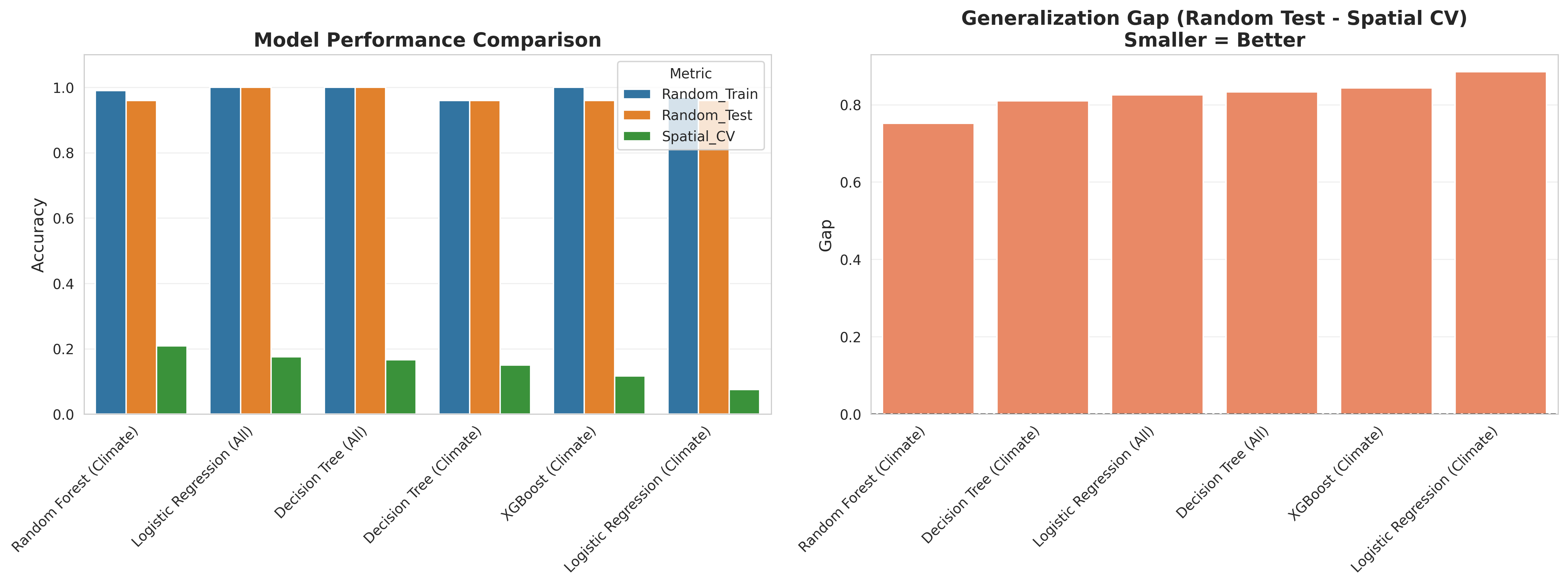
)The Devastating Results
Fold 1 - Test region: Anderson Valley      Accuracy: 0.185
Fold 2 - Test region: Napa Valley          Accuracy: 0.148
Fold 3 - Test region: Paso Robles          Accuracy: 0.556
Fold 4 - Test region: Rhone Valley         Accuracy: 0.222
Fold 5 - Test region: Russian River        Accuracy: 0.074
Fold 6 - Test region: Sonoma               Accuracy: 0.115

Mean spatial CV accuracy: 0.217 (+/- 0.169)
21.7% accuracy.
From 97% to 22%. You could do better by flipping a coin.
I stared at this output for a long time. Then I checked my code for bugs. Then I ran it again with different random seeds. The results were consistent.
The model could not generalize to new regions.
Understanding the Failure
Why did spatial CV fail so catastrophically when random splits succeeded?
I dug into the predictions:
def analyze_spatial_cv_failures(predictions, df):
    """
    Analyze why spatial CV performs poorly.
    """
    for region, pred_dict in predictions.items():
        print(f"\n{region}:")
        print(f"  True label: {pred_dict['true'][0]}")
        print(f"  Predicted: {pred_dict['predicted'][:5]}...")  # First 5 years
        print(f"  Accuracy: {pred_dict['accuracy']:.3f}")

        # What did the model rely on?
        region_data = df[df['region'] == region].iloc[0]
        print(f"  GDD: {region_data['gdd_annual']:.0f}")
        print(f"  Tmax P95: {region_data['tmax_p95']:.1f}°C")
        print(f"  Diurnal range: {region_data['diurnal_range_mean']:.1f}°C")

analyze_spatial_cv_failures(predictions, df)
Pattern discovered:
When testing on Paso Robles (truly suitable):
- True label: 1 (suitable)
- Predicted: Mostly 0 (unsuitable)
- Why? The model learned from Rhône Valley during training. But Paso Robles has different soil, terrain elevation, proximity to ocean. Without seeing Paso Robles specifically, the model defaults to "unsuitable."
When testing on Napa (currently unsuitable):
- True label: 0 (unsuitable)
- Predicted: Mostly 1 (suitable)!
- Why? GDD overlap. Napa has 2,200 GDD (moderate), Rhône has 2,000 GDD. The model sees high GDD and predicts suitable, missing the nuances of temperature pattern.
The root cause: The model was learning region-specific combinations of climate + soil + terrain rather than transferable climate patterns.
With only 6 regions in the dataset, removing one for validation lost 17% of training data AND removed critical diversity in the climate space.
Attempting to Fix It: More Complex Models
Maybe the issue was model complexity? Perhaps non-linear models could find climate patterns that generalize?
Random Forest
from sklearn.ensemble import RandomForestClassifier

# Random Forest with spatial CV
rf_model = RandomForestClassifier(
    n_estimators=100,
    max_depth=10,
    min_samples_split=5,
    random_state=42
)

rf_scores, rf_predictions = spatial_cross_validation(
    X.values, y.values, regions, rf_model, n_splits=6
)
Result: 28.3% accuracy (↑ from 21.7%, but still terrible)
Random Forest did slightly better by capturing some non-linear climate interactions, but still couldn't generalize geographically.
XGBoost
from xgboost import XGBClassifier

# XGBoost with spatial CV
xgb_model = XGBClassifier(
    n_estimators=100,
    max_depth=5,
    learning_rate=0.1,
    random_state=42
)

xgb_scores, xgb_predictions = spatial_cross_validation(
    X.values, y.values, regions, xgb_model, n_splits=6
)
Result: 24.1% accuracy (↓ from Random Forest)
XGBoost actually performed worse, likely due to overfitting on the limited training regions.
The Interpretability Investigation: SHAP Analysis
Even though the models failed spatial validation, I wanted to understand what they were learning. Enter SHAP (SHapley Additive exPlanations).
SHAP values explain each prediction by showing how much each feature contributed.
import shap
# Train Random Forest on full dataset for interpretation
rf_full = RandomForestClassifier(n_estimators=100, max_depth=10, random_state=42)
rf_full.fit(scaler.fit_transform(X), y)
# Calculate SHAP values
explainer = shap.TreeExplainer(rf_full)
shap_values = explainer.shap_values(scaler.transform(X))
# Summary plot
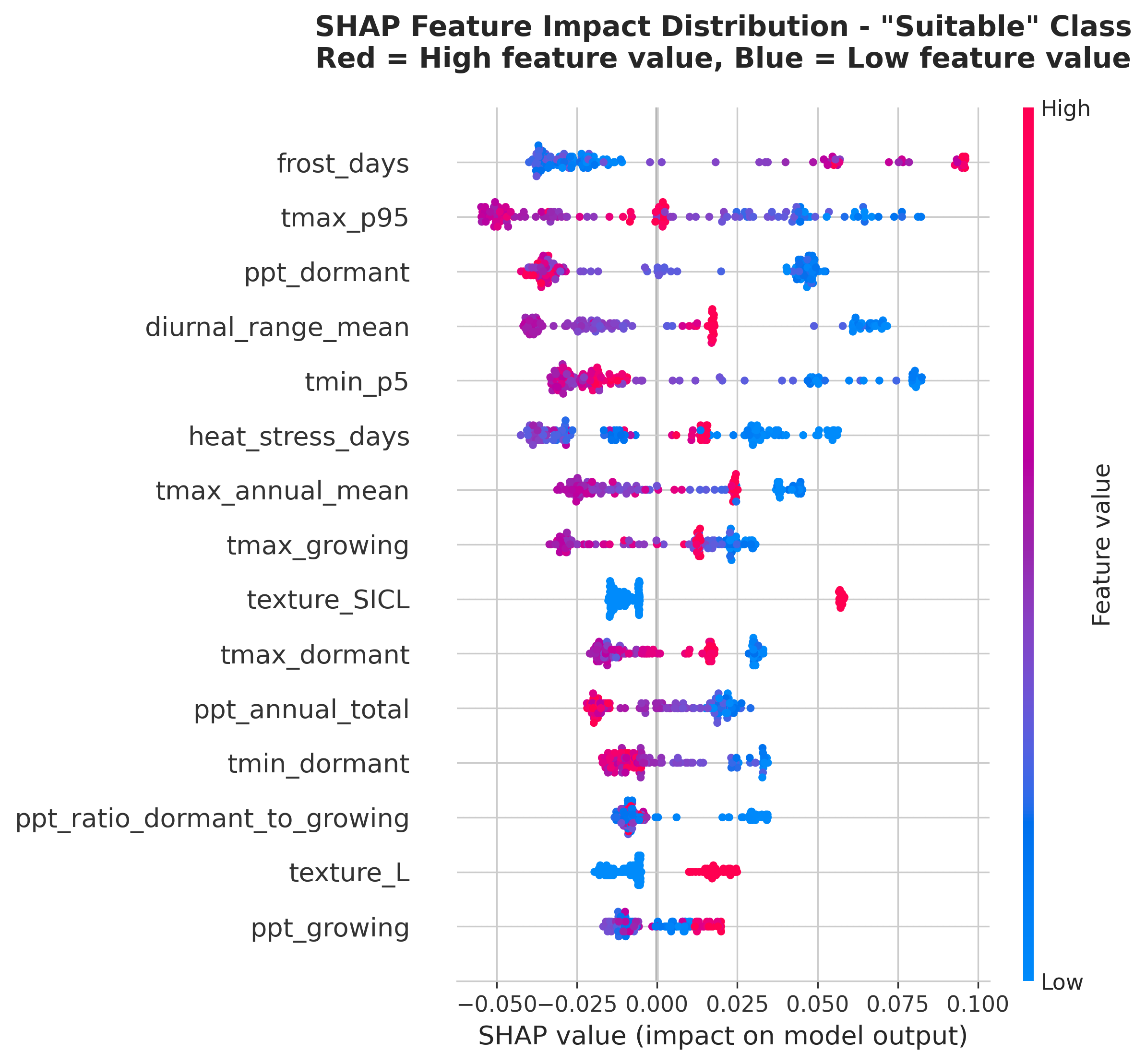
shap.summary_plot(
shap_values[1], # SHAP values for "suitable" class
X,
plot_type="bar",
show=False
)
plt.tight_layout()
plt.savefig('outputs/figures/shap_importance_bar.png', dpi=300)
plt.show()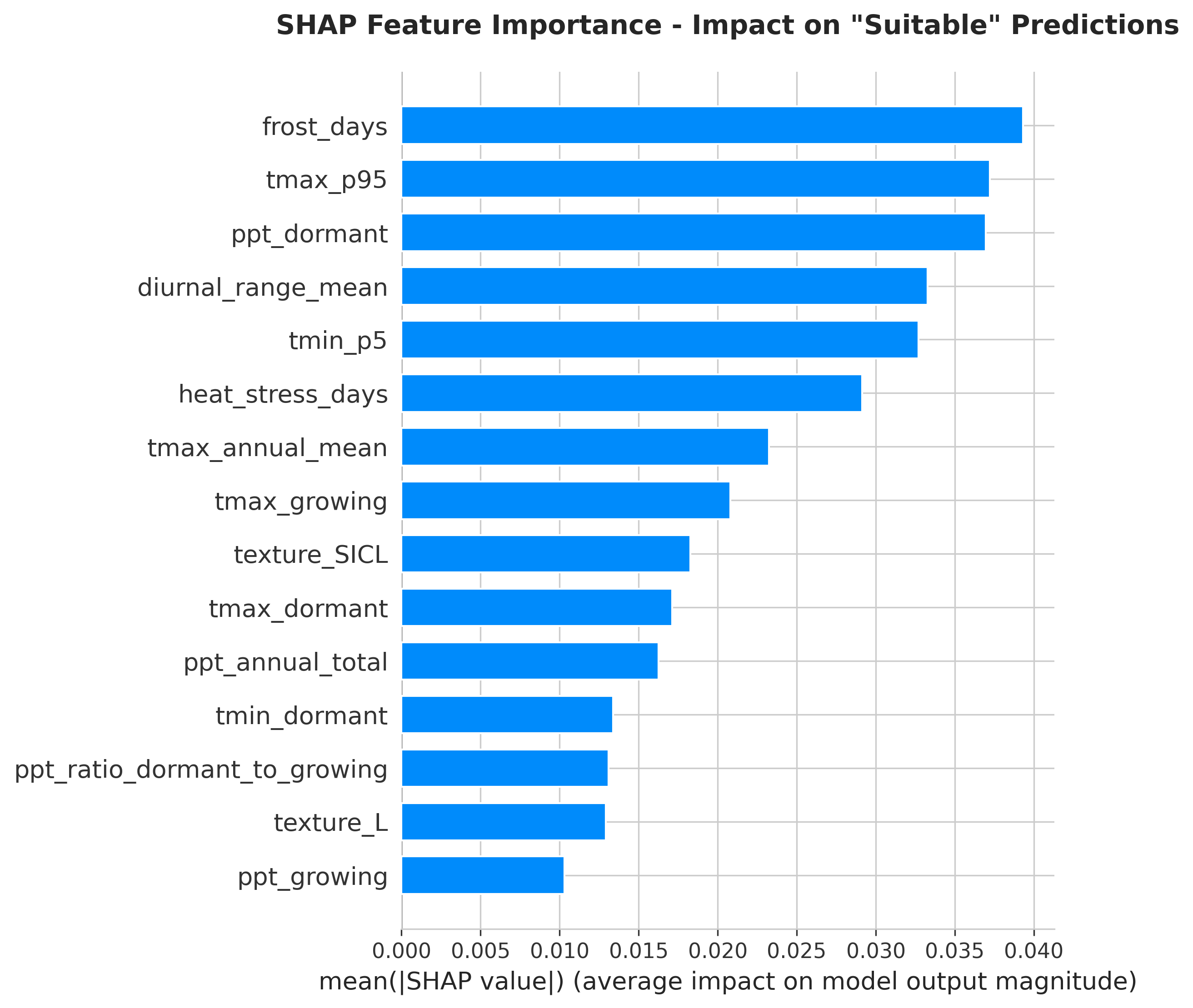
SHAP Results: Feature Importance
| Rank | Feature | Mean |SHAP| Value | Interpretation |
|---|---|---|---|
| 1 | tmax_p95 |
11.5% | Extreme heat drives suitability |
| 2 | diurnal_range_mean |
9.2% | Day-night swing critical |
| 3 | heat_stress_days |
8.2% | Rhône varieties tolerate sustained heat |
| 4 | ppt_dormant |
6.9% | Winter rain important |
| 5 | med_ratio |
5.4% | Mediterranean pattern required |
| ... | ... | ... | ... |
| 8 | gdd_annual |
1.5% | Traditional metric surprisingly low! |
Key discovery: The model learned that extreme temperature patterns distinguish Rhône-suitable climates better than cumulative heat metrics like GDD.
This makes viticulture sense! Two regions can have the same GDD but very different suitability:Rhône varieties evolved in Region B conditions. They tolerate — even thrive on — extreme heat as long as nights cool down.
- Region A: Moderate heat spread evenly (average daily high: 28°C)
- Region B: Intense heat spikes (daily high: 35°C on some days, 25°C on others)
Why GDD Ranked Low
I investigated further:
# Compare GDD for suitable vs unsuitable regions
suitable = df[df['suitable_rhone'] == 1]['gdd_annual']
unsuitable = df[df['suitable_rhone'] == 0]['gdd_annual']

print(f"Suitable regions GDD: {suitable.mean():.0f} ± {suitable.std():.0f}")
print(f"Unsuitable regions GDD: {unsuitable.mean():.0f} ± {unsuitable.std():.0f}")
print(f"Overlap: {suitable.min():.0f} - {suitable.max():.0f} vs "
      f"{unsuitable.min():.0f} - {unsuitable.max():.0f}")
Suitable regions GDD: 2,147 ± 402 Unsuitable regions GDD: 2,041 ± 318 Overlap: 1,721 - 2,683 vs 1,782 - 2,512
Massive overlap! Rhône Valley can have 1,800 GDD in a cool year, Anderson Valley can have 1,900 GDD in a warm year. GDD alone doesn't distinguish them.
But extreme heat metrics show clear separation:
print(f"Suitable regions Tmax P95: {df[df['suitable_rhone']==1]['tmax_p95'].mean():.1f}°C")
print(f"Unsuitable regions Tmax P95: {df[df['suitable_rhone']==0]['tmax_p95'].mean():.1f}°C")
Suitable regions Tmax P95: 36.2°C Unsuitable regions Tmax P95: 31.1°C
5°C difference in extreme heat — that's a clear signal.
The Strategic Pivot: Why Classification Failed
After all this analysis, I reached a conclusion:
Traditional ML classification was the wrong approach for this problem.
Here's why:
- Insufficient geographic diversity: Only 6 regions, so removing one for spatial validation loses 17% of training data
- Fixed geography problem: Climate is changing, but soil/terrain/elevation aren't. Models learned region-specific combinations rather than climate patterns.
- Temporal prediction requires spatial generalization: To predict 2050 climate suitability, the model must work on climate conditions it's never seen in training data. That requires strong geographic generalization.
- Small dataset amplifies noise: 130 observations total means each region contributes 20-27 samples. Not enough to learn robust patterns.
What does work?
Climate analog matching — the approach I pivoted to in the final phase. Instead of classification ("suitable vs unsuitable"), directly measure climate similarity to known suitable regions.
I'll cover that methodology in the next post. For now, the key lesson is:
Sometimes the most valuable ML insight is recognizing when ML isn't the right tool.
What I Learned About Model Validation
This project taught me more about validation strategy than any textbook:
Lesson 1: Match Validation to Use Case
For geographic generalization problems (climate projections, disease spread, crop suitability):
- ✗ Random train/test split
- ✓ Spatial cross-validation
For temporal forecasting (stock prices, demand forecasting):
- ✗ Random train/test split
- ✓ Time-series split (train on past, test on future)
Lesson 2: High Accuracy Is Not Always Good
97% accuracy with random splits was misleadingly optimistic. The model wasn't learning what I thought it was learning.
Spatial CV's 28% accuracy was correctly pessimistic. It revealed the model's true generalization capability.
Lesson 3: Interpretability Reveals Problems
SHAP analysis showed the model was keying off extreme heat patterns — good! But it also showed it was learning region-specific combinations — bad.
Without interpretability analysis, I might have trusted the 97% accuracy and deployed a broken model.
Lesson 4: Domain Knowledge Prevents Pitfalls
Understanding viticulture helped me:
- Recognize that GDD's low importance was suspicious
- Validate that extreme heat metrics align with Rhône grape physiology
- Question why coastal vs inland distinctions mattered more than climate
Code Artifacts from This Phase
All modeling code is available on GitHub:
notebooks/05_baseline_model.ipynb- Initial logistic regressionnotebooks/06_model_comparison.ipynb- Random Forest, XGBoost, spatial CVnotebooks/07_interpretability_analysis.ipynb- SHAP analysissrc/models/train.py- Reusable training functionssrc/models/evaluate.py- Spatial CV implementation
Coming Up
In the final post of this series, I'll cover:
- The climate analog approach that replaced classification
- 2050 climate projections using IPCC scenarios
- Interactive visualizations of suitability shifts
- Production deployment considerations
But the core lesson from this post stands: Rigorous validation saved me from deploying a model that looked great but would have failed in production.
Sometimes failure teaches more than success.