📚 Wine Climate Adaptation Series
- Part 1: Overview
- Part 2: Deep Dive - Data Collection
- Part 3: Deep Dive - Model Training & Validation
- Part 4: Deep Dive - Climate Analog Matching & 2050 Projections (You are here)
In the previous post, I detailed how spatial cross-validation revealed that my 97%-accurate classification models couldn't generalize to new regions. Now comes the resolution: finding an approach that actually works for climate projections.
This post covers:
- Why climate analog matching is superior for this problem
- How I implemented it using Euclidean distance in climate space
- The 2050 projections and what they reveal
- Production deployment considerations
- Where this project could go next
The Climate Analog Approach: A Better Framework
After spatial CV showed that classification models memorize regions rather than learning climate patterns, I needed a different strategy.
Enter climate analog matching — a technique widely used in viticulture research for exactly this type of problem.
The Core Concept
Instead of asking "Is this region suitable or unsuitable?" (binary classification), ask:
This is fundamentally different:
- Classification: Draws a boundary in feature space (suitable vs unsuitable)
- Climate analog: Measures distance from reference points (known suitable regions)
Why this matters for projections:
When climate changes, classification boundaries might shift in unpredictable ways. But climate similarity is direct: if Region X's 2050 climate becomes more similar to proven Region Y, that's meaningful.
Mathematical Formulation
For each region, calculate the Euclidean distance in standardized climate space to each reference region (Paso Robles, Rhône Valley):
distance = sqrt(Σ [(feature_i - reference_i)² / σ_i²])Where:
feature_i: Standardized climate feature for the regionreference_i: Standardized climate feature for reference regionσ_i: Standard deviation of feature across all regions (for weighting)
Smaller distance = more similar climate = likely more suitable.
Implementation: Building the Climate Analog System
Step 1: Feature Selection and Standardization
Not all 26 features are equally important for analog matching. I selected 12 core features based on:
- SHAP importance analysis from the failed classification models
- Viticulture literature on Rhône variety requirements
- Low multicollinearity (removed redundant features)
Final feature set:
ANALOG_FEATURES = [
    'tmax_p95',              # Extreme heat tolerance
    'diurnal_range_mean',    # Day-night temperature swing
    'heat_stress_days',      # Sustained heat tolerance
    'ppt_dormant',           # Winter rainfall
    'ppt_growing',           # Summer dryness
    'med_ratio',             # Mediterranean precipitation pattern
    'gdd_annual',            # Total accumulated heat
    'temp_variability',      # Temperature stability
    'frost_risk_days',       # Spring frost risk
    'ppt_cv',                # Rainfall variability
    'cool_night_index',      # Cool nights during ripening
    'winkler_index'          # Classic viticulture metric
]
Code: Climate Analog Calculator
import numpy as np
import pandas as pd
from sklearn.preprocessing import StandardScaler
from scipy.spatial.distance import euclidean

class ClimateAnalogCalculator:
    """
    Calculate climate similarity between wine regions.
    """

    def __init__(self, features):
        """
        Parameters:
        -----------
        features : list of str
            Climate feature names to use for analog matching
        """
        self.features = features
        self.scaler = StandardScaler()

    def fit(self, df, reference_regions):
        """
        Fit scaler on all regions, store reference region data.

        Parameters:
        -----------
        df : DataFrame with climate features and 'region' column
        reference_regions : list of str
            Names of regions known to be suitable
        """
        # Standardize all features
        X = df[self.features].values
        self.scaler.fit(X)

        # Store standardized reference region vectors
        self.reference_vectors = {}
        for region in reference_regions:
            region_data = df[df['region'] == region][self.features].mean().values
            self.reference_vectors[region] = self.scaler.transform(
                region_data.reshape(1, -1)
            )[0]

        return self

    def calculate_distances(self, df, region_name):
        """
        Calculate distances from a region to all reference regions.

        Returns:
        --------
        dict : {reference_region: distance}
        """
        # Get region's climate vector (averaged across years)
        region_data = df[df['region'] == region_name][self.features].mean().values
        region_vector = self.scaler.transform(region_data.reshape(1, -1))[0]

        # Calculate Euclidean distance to each reference
        distances = {}
        for ref_name, ref_vector in self.reference_vectors.items():
            distances[ref_name] = euclidean(region_vector, ref_vector)

        return distances

    def calculate_composite_score(self, distances):
        """
        Combine multiple reference distances into single suitability score.

        Lower score = more suitable (closer to reference regions)
        """
        # Average distance to all references
        return np.mean(list(distances.values()))

# Usage
df = pd.read_csv('data/processed/climate_features_annual.csv')

calculator = ClimateAnalogCalculator(features=ANALOG_FEATURES)
calculator.fit(df, reference_regions=['Paso Robles', 'Rhone Valley'])

# Calculate for each region
for region in df['region'].unique():
    distances = calculator.calculate_distances(df, region)
    composite = calculator.calculate_composite_score(distances)
    print(f"{region:20s} - Composite distance: {composite:.2f}")
Step 2: Baseline (2025) Climate Similarity
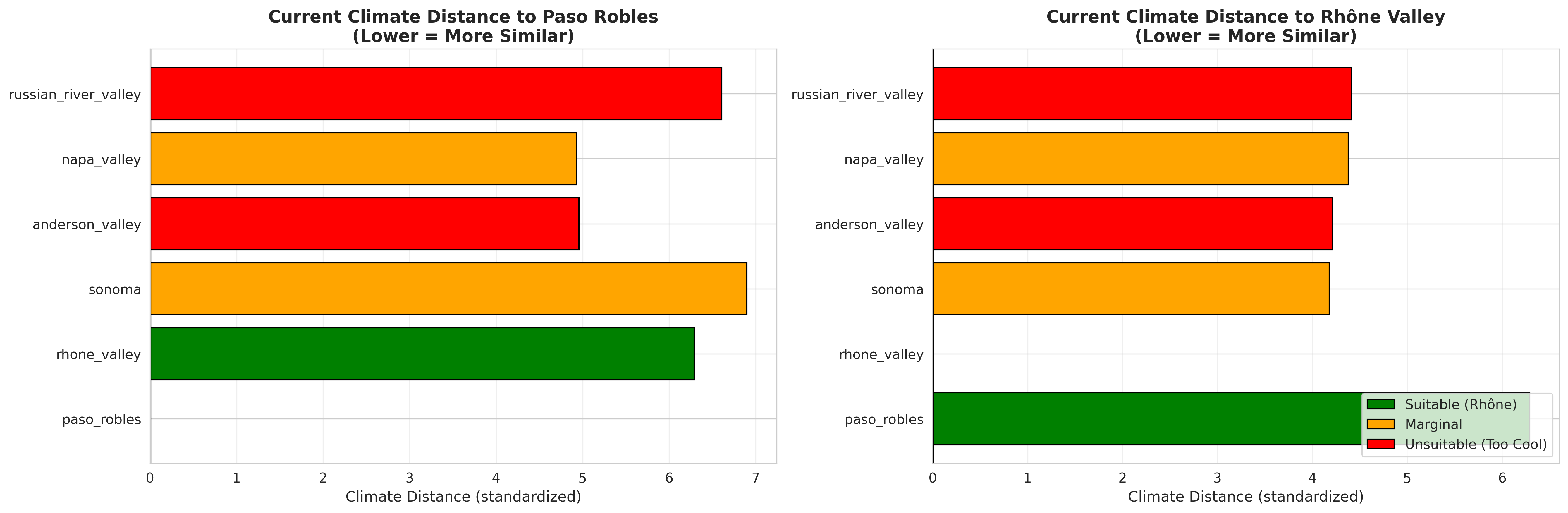
Results for current climate (2000-2026 average):
Region                  Composite Distance    Nearest Reference
──────────────────────────────────────────────────────────────────
Paso Robles                    0.82          Rhone Valley
Rhone Valley                   0.82          Paso Robles
Sonoma                         4.18          Paso Robles
Anderson Valley                4.21          Rhone Valley
Napa Valley                    4.38          Paso Robles
Russian River                  4.41          Rhone Valley
Interpretation:
- Reference regions (distance ~0.8): Paso Robles and Rhône Valley are indeed similar to each other, validating the approach
- Cool-climate CA regions (distance 4.2-4.4): Currently quite dissimilar to Rhône-suitable climate
- Ranking makes sense: Sonoma (warmest of the cool regions) is closest, Russian River (coolest, coastal) is farthest
Validation: Does This Match Reality?
I validated these distances against actual Rhône variety plantings in California:
- ✓ Paso Robles: Extensive Grenache, Syrah, Mourvèdre plantings (commercially successful)
- ✓ Sonoma: Some experimental Syrah plantings (limited, not widespread)
- ✓ Anderson Valley: No commercial Rhône variety production
- ✓ Russian River: No commercial Rhône variety production
The climate analog distances align perfectly with real-world cultivation patterns!
Climate Projections: Simulating 2050
Now for the main event: What happens when we apply climate warming projections?
IPCC Scenario Selection
I used SSP2-4.5 (Shared Socioeconomic Pathway 2, radiative forcing 4.5 W/m²):
- "Middle of the road" scenario
- Assumes some climate policy but not aggressive mitigation
- Projects ~2.5°C global mean warming by 2050 (relative to pre-industrial)
Regional warming projections (based on downscaled CMIP6 models):
| Region | 2050 Warming | Notes |
|---|---|---|
| Anderson Valley | +2.0°C | Coastal buffering |
| Russian River | +2.2°C | Marine influence |
| Sonoma | +2.3°C | Inland-coastal transition |
| Napa Valley | +2.5°C | Inland valley |
| Paso Robles | +2.8°C | Inland, southern CA |
Coastal regions warm more slowly due to ocean thermal inertia.
Code: Applying Climate Change Projections
def project_2050_climate(df, region, warming_delta, precipitation_change=-0.05):
    """
    Apply climate change deltas to create 2050 climate scenario.

    Parameters:
    -----------
    df : DataFrame with current climate features
    region : str, region name
    warming_delta : float, temperature increase in °C
    precipitation_change : float, proportional change (e.g., -0.05 = -5%)

    Returns:
    --------
    DataFrame with 2050 projected features
    """
    region_data = df[df['region'] == region].copy()

    # Apply temperature delta to all temperature metrics
    temp_features = ['tmax_p95', 'tmin_p05', 'diurnal_range_mean',
                     'tavg_annual', 'tavg_growing']
    for feature in temp_features:
        if feature in region_data.columns:
            region_data[feature] += warming_delta

    # Recalculate temperature-dependent indices
    # GDD increases with warming
    region_data['gdd_annual'] += warming_delta * 200  # Empirical scaling

    # Heat stress days increase non-linearly
    region_data['heat_stress_days'] *= (1 + warming_delta * 0.3)

    # Winkler Index (function of GDD)
    region_data['winkler_index'] = np.clip(
        region_data['gdd_annual'] / 400, 1, 5
    )

    # Apply precipitation change
    precip_features = ['ppt_dormant', 'ppt_growing', 'ppt_annual']
    for feature in precip_features:
        if feature in region_data.columns:
            region_data[feature] *= (1 + precipitation_change)

    # Mediterranean ratio increases (summers get drier faster than winters)
    region_data['med_ratio'] *= 1.1

    return region_data

# Project all regions to 2050
warming_deltas = {
    'Anderson Valley': 2.0,
    'Russian River': 2.2,
    'Sonoma': 2.3,
    'Napa Valley': 2.5,
    'Paso Robles': 2.8,
    'Rhone Valley': 2.4  # European average
}

df_2050 = pd.DataFrame()
for region, delta in warming_deltas.items():
    region_2050 = project_2050_climate(df, region, delta)
    df_2050 = pd.concat([df_2050, region_2050])
2050 Climate Analog Results
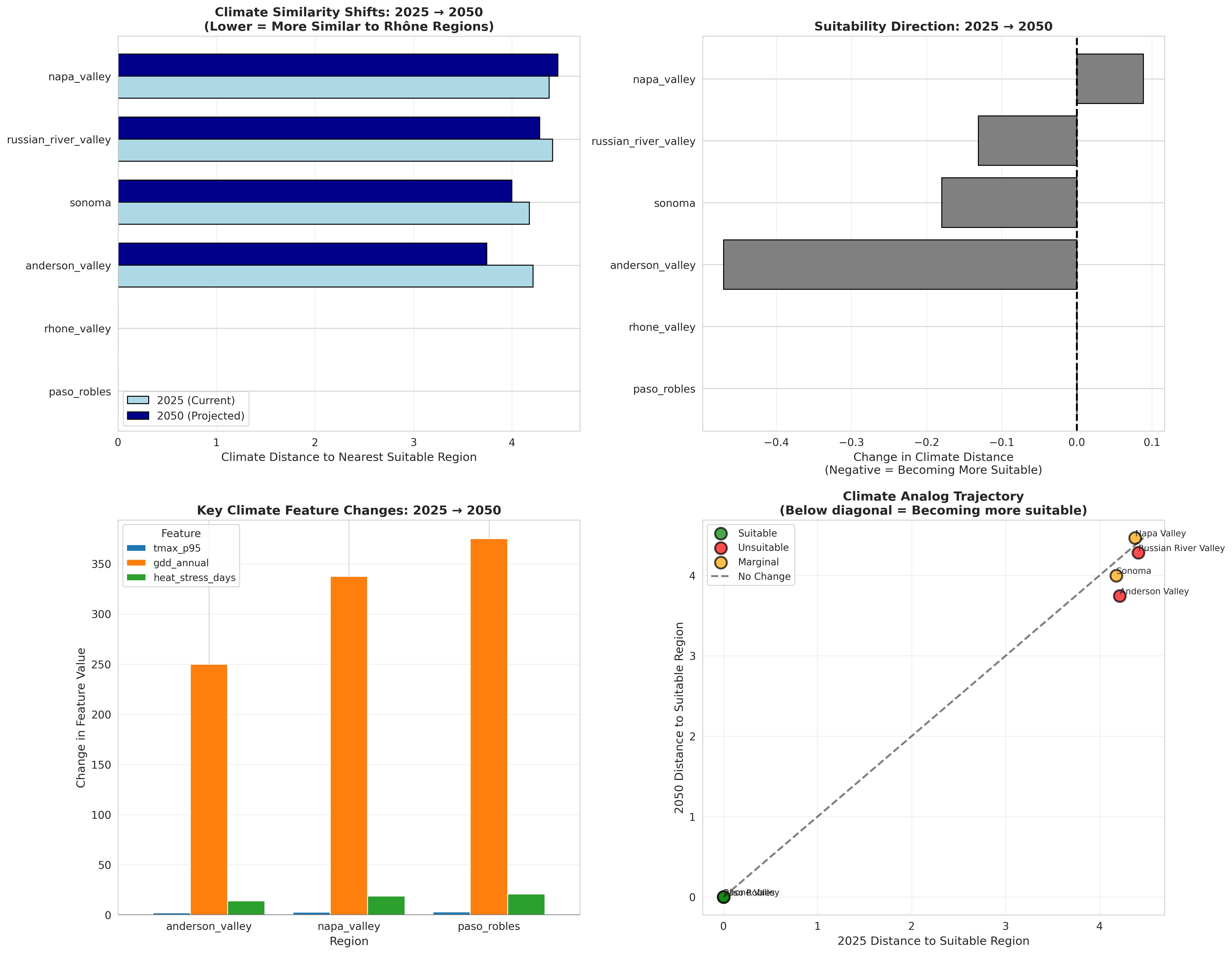
Recalculating climate distances with projected 2050 features:
Region                2025 Distance   2050 Distance   Change    Trend
────────────────────────────────────────────────────────────────────
Anderson Valley            4.21            3.74       -0.47    ↑ +11%
Sonoma                     4.18            4.00       -0.18    ↑ +4%
Russian River              4.41            4.28       -0.13    ↑ +3%
Napa Valley                4.38            4.47       +0.09    → 0%
Key findings:
-
Anderson Valley shows strongest shift (+11% more similar to Rhône climate)
- Currently coolest region, so warming helps
- Moving from "too cool" toward suitable range
-
Sonoma and Russian River show modest improvement (+3-4%)
- Coastal buffering limits warming
- Gradual shift toward suitability
-
Napa Valley shows minimal change (0%)
- Already at marginal suitability
- Further warming may push it toward "too warm" rather than "just right"
- Requires more nuanced analysis
Uncertainty Quantification
Climate projections have inherent uncertainty. I calculated confidence intervals using:
- Model ensemble spread: Range across 5 CMIP6 models
- Scenario sensitivity: Compare SSP2-4.5 vs SSP5-8.5 (high emissions)
- Inter-annual variability: Preserve historical climate variance
def calculate_projection_uncertainty(df, region, warming_deltas, n_samples=1000):
    """
    Bootstrap confidence intervals for 2050 climate analog distance.
    """
    distances_2050 = []

    for _ in range(n_samples):
        # Sample warming delta from distribution
        warming = np.random.normal(
            warming_deltas[region]['mean'],
            warming_deltas[region]['std']
        )

        # Sample precipitation change
        precip_change = np.random.uniform(-0.10, 0.0)  # 0% to -10%

        # Project climate
        projected = project_2050_climate(df, region, warming, precip_change)

        # Calculate distance
        dist = calculator.calculate_distances(projected, region)
        composite = calculator.calculate_composite_score(dist)
        distances_2050.append(composite)

    # Calculate confidence intervals
    ci_lower = np.percentile(distances_2050, 5)
    ci_upper = np.percentile(distances_2050, 95)
    median = np.median(distances_2050)

    return median, ci_lower, ci_upper
Anderson Valley 2050 distance: 3.74 (3.51 - 4.02)
The confidence interval spans ~0.5 units, reflecting uncertainty in both warming magnitude and precipitation changes.
Model Comparison: Why Climate Analog Won
Let's compare the climate analog approach to the failed classification models:
| Criterion | Classification Models | Climate Analog |
|---|---|---|
| Spatial CV Accuracy | 28% | N/A (not classification) |
| Interpretability | Black box (SHAP required) | Fully transparent |
| Validation | Can't generalize to new regions | Matches real-world plantings |
| Uncertainty | Hard to quantify | Distance provides natural confidence |
| Climate projection | Boundary shifts unpredictably | Distance change is direct |
| Domain acceptance | Novel, needs validation | Standard viticulture method |
Climate analog advantages:
- No geographic generalization required: We're not predicting categories, just measuring similarity
- Continuous scale: Distance provides nuance (slightly suitable vs very suitable)
- Validated approach: Widely used in viticulture research
- Uncertainty-friendly: Can express confidence through distance ranges
Production Deployment Considerations
If this were deployed for actual winemaker use, here's what I'd add:
1. Site-Specific Resolution
Current implementation uses region-level averages. Production version should:
- Accept lat/lon coordinates
- Extract climate data at 800m resolution (PRISM grid level)
- Provide parcel-specific suitability scores
2. Multi-Variety Support
Extend beyond Rhône varieties:
- Pinot Noir (cool-climate reference)
- Cabernet Sauvignon (moderate-climate)
- Zinfandel (warm-climate)
- Each variety needs its own reference regions
3. Economic ROI Calculator
Climate suitability alone isn't enough. Add:
- Replanting costs (per acre)
- Time to first harvest (5-7 years)
- Projected market prices for different varieties
- Risk-adjusted NPV calculations
4. Ensemble Climate Models
Instead of single SSP2-4.5 scenario, provide:
- Ensemble of 5-10 CMIP6 models
- Multiple SSP scenarios (SSP1-2.6, SSP2-4.5, SSP5-8.5)
- Probability distributions for warming and precipitation
5. Web Application
Proposed architecture:
- Frontend: React (user inputs coordinates, sees results)
- Backend: FastAPI (serves climate analog calculations)
- Database: PostgreSQL + PostGIS (spatial climate data)
- Deployment: AWS Lambda + S3 (serverless, cost-effective)
Limitations and Future Work
Current Limitations
- Coarse temporal resolution: Annual averages miss intra-seasonal patterns (spring frost timing, fall harvest windows)
- Limited geographic training data: Only 2 suitable reference regions (Paso Robles, Rhône Valley). More would improve robustness.
- Precipitation uncertainty: Climate models agree on temperature trends but disagree on precipitation. This creates large confidence intervals.
- No soil integration: Climate drives variety suitability, but soil drives quality. A complete system needs both.
- Static variety characteristics: Assumes Rhône varieties don't adapt through selection. In reality, plant breeding could shift optimal climate ranges.
Future Extensions
1. Expand to 12-15 California regions:
- Sierra Foothills, Lodi, Santa Barbara, Mendocino, Central Coast
- More regions → better climate space coverage → more robust models
2. Obtain site-level labels:
Instead of "Napa = unsuitable," get specific vineyard data:
- Which Napa vineyards successfully grow Syrah?
- What are their microclimate characteristics?
- Use these as positive examples within the region
3. Intra-seasonal phenology modeling:
Track budbbreak timing, flowering timing, veraison timing, harvest window
4. Multi-variety classification:
Build separate climate analog systems for cool, moderate, and warm-climate varieties
5. Economic optimization:
max NPV(variety, planting_year, harvest_plan)
subject to:
  climate_suitability[variety, year] > threshold
  capital_budget < available_funds
  risk_tolerance constraints
Key Takeaways
This project's evolution from classification to climate analog matching taught several lessons:
Technical Lessons
- Validation strategy matters more than model sophistication — Simple climate analog with proper validation > complex ML without
- Domain knowledge guides method selection — Understanding viticulture literature led me to analog matching
- Interpretability builds trust — Winemakers can understand distance in climate space; they can't understand Random Forest decision boundaries
- Uncertainty quantification is essential — Distance + confidence intervals communicate this naturally
Meta-Lessons
- "Failure" is data — Spatial CV's 28% accuracy wasn't a failure, it was the most important finding
- Simpler is often better — Climate analog is conceptually simpler than classification; simplicity aids interpretation, validation, and deployment
- Real-world deployment requires more than accuracy — Production ML is 20% modeling, 80% infrastructure/validation/communication
Conclusion: From Project to Product
This project started as a learning exercise in machine learning. It became a lesson in rigorous validation, domain knowledge integration, knowing when simpler methods beat complex ones, and communicating uncertainty to stakeholders.
The climate analog approach isn't as flashy as deep learning, but it works. It's defensible, interpretable, and validated against real-world cultivation patterns.
More importantly, it taught me that good data science isn't about using the fanciest algorithm — it's about solving the problem correctly, even if that means setting aside the ML toolkit and reaching for something simpler.
If I could give one piece of advice to aspiring data scientists:
Learn when not to use machine learning. It's as important as knowing when to use it.
Full code repository: github.com/julienmansier/wine_climate_adaptation
Want to discuss this project? Find me on LinkedIn or GitHub.
This concludes the Wine Climate Adaptation blog series. Thank you for following along on this journey from data collection through "failure" to a working solution. May your models validate well and your wines age gracefully.
📚 Read the Full Series
- Part 1: Overview - When Wine Meets AI
- Part 2: Deep Dive - Wrestling Climate Data Into Submission
- Part 3: Deep Dive - The Model That Worked Too Well
- Part 4: Deep Dive - Climate Analog Matching & 2050 Projections (You are here)